Multivariate drift detection using Domain Classifier with a Python tutorial

Do not index

Canonical URL

Introduction

You’ve identified a problem you want to tackle with machine learning (ML), acquired the data, and meticulously analyzed and preprocessed it. You’ve built a robust model that performs well on several evaluation metrics. While one might hope for a fairy-tale ending where the model predicts flawlessly ever after, it's likely that its performance will degrade over time. Therefore, it's crucial to proactively monitor your model's performance in production to maximize its utility.

Fortunately, there are many methods for monitoring your model's performance. Once you have identified a drop in your model's performance, you need to figure out what caused it. That’s where detecting data drift comes into the picture.

Covariate shift is a type of data drift related to ML models' input features. Techniques to detect covariate shifts can generally be categorized into univariate and multivariate drift methods. In this article, we take a deeper look at the Domain Classifier method, which we’ve just added to NannyML OSS.

The method is a great tool for detecting multivariate drift. We offer insight into its rationale, provide a detailed explanation of its functioning, and give a straightforward, practical guide on implementing it using the NannyML OSS library with just a few lines of Python code.

Data drift in a nutshell

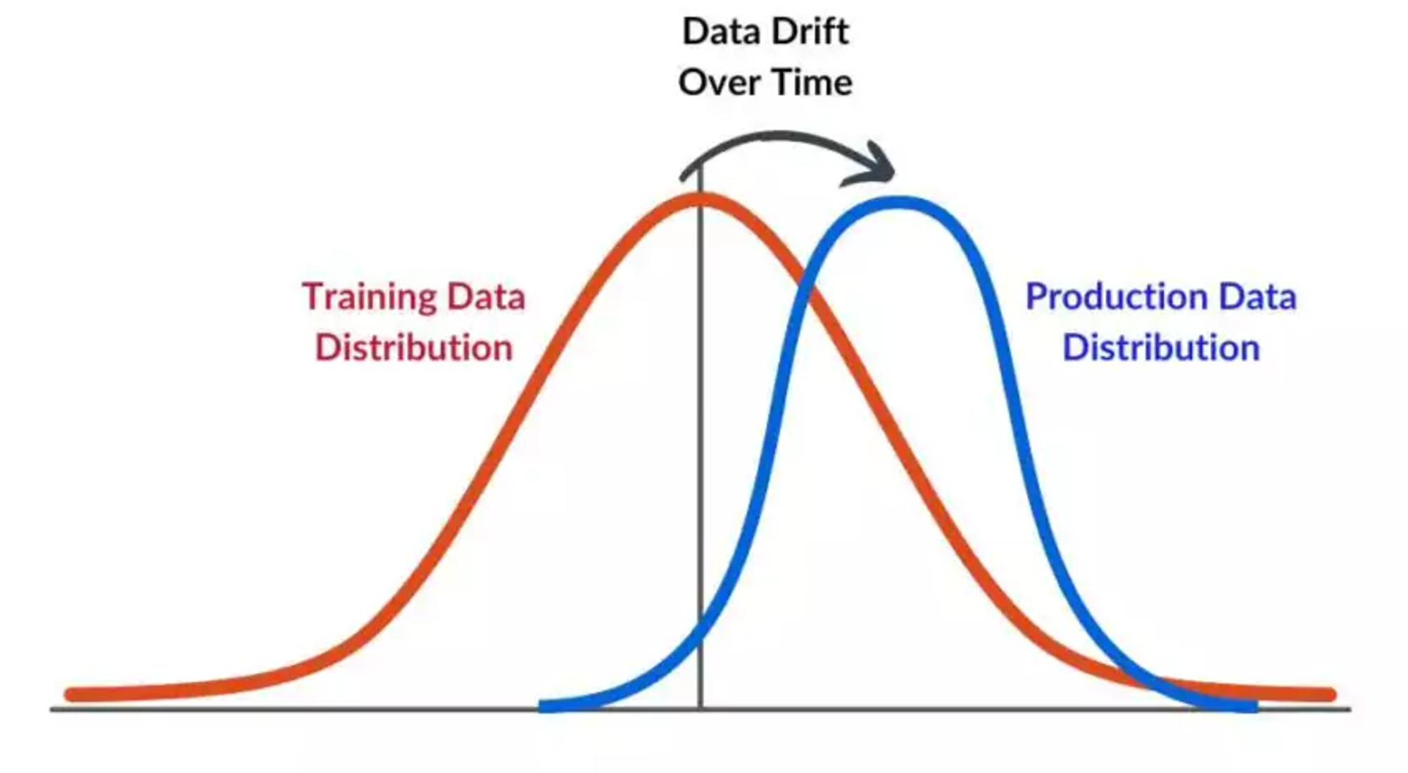
Covariate shift is a specific type of data drift that refers to the phenomenon wherein the statistical properties of the data used to train a machine learning model change over time. Such changes can result in a decline in the model's performance. For instance, a model that initially performed well upon deployment might experience a decrease in accuracy as the distribution of one or more features shifts over time.

Here’s a more concrete example: Imagine an e-commerce company trains an ML model to predict the traffic to its website to determine staffing requirements for customer service. They are using historical data to train their model, and one of the input features considered is the source of traffic (social media, direct traffic, organic search, etc.). However, after deploying their model to production to make predictions, they launched a huge marketing campaign, which increases social media traffic. This changes the distribution of the input feature. This is an occurrence of covariance shift, and it could be the cause of a degradation of the model’s predictions on new data.

Image taken from Spot Intelligence: https://spotintelligence.com/2024/04/08/data-drift-in-machine-learning/

Univariate drift refers to changes in the distribution of a single feature used to train an ML model. Several methods employed to detect univariate drift are based on statistical tests such as the Kolmogorov-Smirnov test or the Chi-squared test. Other approaches are based on divergence measures such as the Jensen-Shannon divergence.

While techniques for detecting univariate drift are relatively straightforward, they might overlook relationship changes between features. That is, while the distributions of individual features remain unchanged, their joint distributions might have shifted. This is why we need multivariate drift methods to identify changes in the joint distributions of some or all features.

The above image illustrates a multivariate drift between two datasets without univariate drifts. The top row shows the marginal distributions of and (left) and their joint distribution (right) for the first dataset. The bottom row displays the same for the second dataset.

The marginal distributions of and remain practically unchanged, as seen in the overlapping density curves of both datasets. However, the joint distributions differ significantly. This example demonstrates how the relationship between variables can change (multivariate drift) even when their individual distributions do not.

NannyML has devised two methods to help data scientists detect multivariate drift when it occurs. The first method employs Principal Component Analysis (PCA) and is extensively discussed with a practical example in another article on NannyML’s blog. The second approach, known as the Domain Classifier, is the focus of this article.

How the Domain Classifier method works

The Domain Classifier method detects multivariate drift by assessing to what extent new data used to make predictions (monitored data) differs from data on which the model's performance is assumed to be stable and accurate (reference data).

It accomplishes this by training a LightGBM binary classifiers on the reference and monitored data. It then relies on the AUROC score (sometimes called to ROC AUC score) as a metric for how easily the classifier can distinguish between reference data and monitored data. If it is easy to discriminate between reference and monitored data, it indicates multivariate drift. This method can effectively capture drifts in the joint probability of some or all the features used to train an ML model.

The AUROC score and how it helps us detect multivariate drift

The receiver operating characteristic (ROC) is a graphical plot that illustrates the true positive rate (TPR) against the false positive rate (FPR) of a classification model at various threshold settings. It is used to showcase the performance of binary classifiers across different classification threshold values and assumes a value between 0 and 1, where 1 indicates a perfect classifier and 0.5 indicates a random classifier. For an intuitive explanation of the method, you can watch the StatQuest video by the legendary Josh Starmer.

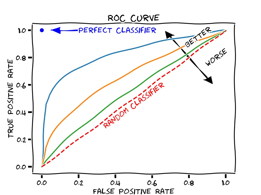
Image by Martin Thoma: https://commons.wikimedia.org/wiki/File:Roc-draft-xkcd-style.svg#filelinks

A higher AUROC score means it is easier to discriminate between the monitored and the reference data, indicating greater differences between them. Therefore, an AUROC score closer to 1 suggests a possible multivariate drift. The Domain Classifier calculates the AUROC score for each data chunk and triggers an alert if it exceeds a certain threshold (by default, the range is [0.45, 0.65]), although this threshold can be customized.

Data chunks are crucial for monitoring in NannyML, as all results are generated at the chunk level. Here’s a definition of what a data chunk is: A data chunk is simply a sample of data, with each chunk representing a single data point in the monitoring results. Chunks are usually created based on time periods, containing all observations and predictions from a specific interval, such as an hour, day, or month. They can also be size-based, where each chunk contains a fixed number of observations, or number-based, where the entire dataset is split into a predetermined number of chunks.

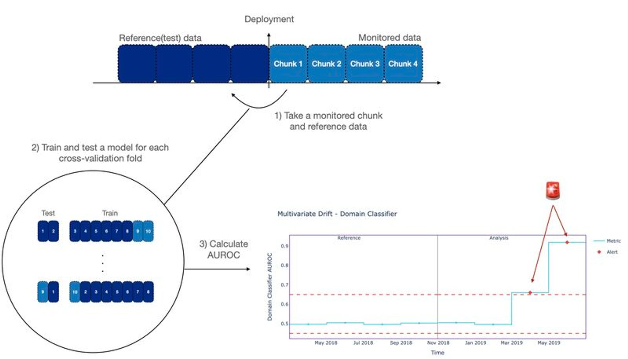
A recap of the Domain Classifier method, step by step

Take as input the reference data, the monitored data and a chunking parameter.

The reference data is considered class 0, the monitored data is class 1.

For each data chunk:

Train a LightGBM binary classifier using stratified k-fold cross-validation.

Calculate the cross-validated AUROC score for the binary classifier.

If the AUROC score exceeds a predefined threshold (e.g., 0.65), an alert is raised to indicate a potential multivariate data drift.

Now that we’ve covered how it works, let’s take a look at it in action…

A practical example in Python

We will implement the Domain Classifier in Python using the NannyML OSS package. We will use the Weather Prediction dataset (courtesy of the Shifts Project) as a working example. Covariate shift often occurs in weather data due to seasonal weather changes. You can follow along as we code and use the provided notebook.

While the complete dataset is available at the link above, we will focus only on the data from September and October for this tutorial. You can download the specific datasets from the following links: 🔗 September Data | 🔗 October Data

Note that in the data at the above link, the timestamp has already been processed to be in the correct DateTime format, and the data has been sorted according to the timestamp.

We kick things off by importing the NannyML package and other necessary libraries. We then proceed to import the data.

# Install the NannyML library using pip
%pip install nannyml

# Import necessary libraries
import nannyml as nml
import pandas as pd
import numpy as np
import matplotlib.pyplot as plt

from google.colab import drive

# Mount Google Drive
drive.mount('/content/drive')

# Read the CSV files into pandas DataFrames
# Note: you might need to adjust the path depending on where the data is stored
reference_df = pd.read_csv("/content/drive/My Drive/Colab Notebooks/domain_classifier_tutorial/september_data.csv")
monitored_df = pd.read_csv("/content/drive/My Drive/Colab Notebooks/domain_classifier_tutorial/october_data.csv")

# Work with a subset of the dataset
reference_df = reference_df.tail(20_000)
monitored_df = monitored_df.head(20_000)

We then conduct some basic exploratory data analysis to gain a better understanding of the data we're working with.

# Create a summary table for September
reference_summary_table = pd.DataFrame({
  'Column Name': reference_df.columns.tolist(),
  'Data Type': reference_df.dtypes.tolist(),
  'Number of Missing Values': reference_df.isnull().sum().tolist(),
  'Number of Unique Values': reference_df.nunique().tolist()
})

# Create a summary table for October
monitored_summary_table = pd.DataFrame({
  'Column Name': monitored_df.columns.tolist(),
  'Data Type': monitored_df.dtypes.tolist(),
  'Number of Missing Values': monitored_df.isnull().sum().tolist(),
  'Number of Unique Values': monitored_df.nunique().tolist()
})

# Display the summary tables
def display_summary(title, df, summary_table):
    from IPython.display import display, HTML

    html_title = f"<h2>{title}</h2>"
    html_entries = f"<p><strong>Number of entries in the DataFrame:</strong> {df.shape[0]}</p>"
    html_table = summary_table.to_html(classes='summary-table', index=False)

    display(HTML(html_title + html_entries + html_table))

# Display for September
display_summary("Reference data (September Data)", reference_df, reference_summary_table)

# Display for October
display_summary("Monitored data (October Data)", monitored_df, monitored_summary_table)

We want to clean our data to ensure the Domain Classifier performs well. We remove columns with many missing values and disregard those features in our analysis.

# List of features to be dropped from the datasets
features_to_drop = ['wrf_t2', 'wrf_t2_next', 'wrf_psfc', 'wrf_rh2', 'wrf_wind_u', 'wrf_wind_v', 'wrf_rain', 'wrf_snow', 'wrf_graupel', 'wrf_hail', 'wrf_t2_interpolated', 'wrf_t2_grad']

# Remove the specified columns from the reference DataFrame
reference_df.drop(columns=features_to_drop, inplace=True)

# Remove the specified columns from the monitored DataFrame
monitored_df.drop(columns=features_to_drop, inplace=True)

Finally, we use the DomainClassifierCalculator method from the NannyML OSS package to detect multivariate drift and visualize the results. This method can be further parametrized, as outlined in the documentation.

# Set the threshold for raising data drift alert
constant_threshold = nml.thresholds.ConstantThreshold(lower=0.45, upper=0.75)

# Initialize multivariate drift calculator with Domain Classifier
dcc = nml.DomainClassifierCalculator(
    feature_column_names=reference_df.columns.drop('timestamp'),
    timestamp_column_name='timestamp',
    chunk_size=1_000,
    hyperparameters={'n_estimators': 50,
                     'learning_rate': 1.0,
                     'max_depth': 3,
                     'random_state': 42},
    threshold=constant_threshold
)

# Fit the multivariate drift calculator on the reference data
dcc.fit(reference_df)

# Calculate drift on the production data
multivariate_drift_results = dcc.calculate(monitored_df)

# Plot the multivariate drift results
figure = multivariate_drift_results.plot()
figure.show()

Graphical representation of the Domain Classifier’s output

We observe that the AUROC score for the reference data fluctuates around 0.5 and falls within the threshold that indicates there is no data drift (shown with a dotted red line in the above figure). The production data, however, has an AUROC score closer to 1, which means this data is easily distinguishable from the reference data, an indication of multivariate drift.

More about the parametrization

It is important to note that the way we parameterize the chunk size significantly impacts the performance of the Domain Classifier. If the chunks are too small, they might capture noise, and the AUROC will consistently fall out of the threshold, which, of course, is not practical as it would lead to many false alerts. However, if the chunks are too large, we might not get enough fine-grained results, which might result in multivariate drift going undetected for a long time.

Like with many things, it is a tradeoff, and finding the right chunk size can take a bit of playing around. In the above-mentioned results, we set chunk_size = 1_000. Below is an example of the Domain Classifier results where the chunk size is too small. Here, chunk_size = 100.

Graphical representation of the Domain Classifier’s results with a chunk size that is too small

In the above example, we also see that we tune the hyperparameters of the LightGBM classifier, which the Domain Classifier method uses. The reason we do this is because the results obtained using the Domain Classifier with the default parameters resulted in classifiers that were too strong. They could too easily distinguish between each chunk. Thus, we had to limit its learning capacity.

The hyperparameters used in this example were obtained by performing a systematic grid search and trying out different values. The code for the grid search is included in the provided notebook.

The upper threshold for raising alerts is set to 0.65 by default but depends on the user’s knowledge of their data and understanding of the context. In our example, we deal with weather data, which can fluctuate over short periods of time. Therefore, we parameterize the upper threshold to 0.75 to achieve the desired results. In general, if you are dealing with data with a lot of small changes that the Domain Classifier might pick up on, the best approach is to raise the upper threshold.

Although data drift detection is a powerful and crucial part of post-deployment ML, its presence may or may not directly affect the model's performance. NannyML has developed methods for monitoring models that can mitigate false alarms of declining model performance. Even better, these methods don’t rely on ground truth. Intrigued? Explore the following articles for a detailed explanation.

Don't be Fooled by Data Drift | ML Monitoring Tools

While being a key component of a healthy monitoring workflow, data drift is a suboptimal alerting tool. Not all data drift impacts model performance.

https://www.nannyml.com/blog/when-data-drift-does-not-affect-performance-machine-learning-models

No Ground Truth: How to Monitor ML Models

Learn how monitoring machine learning models is possible without access to target data. Understand nannyML Performance Estimation algorithm.

https://www.nannyml.com/blog/model-monitoring-without-ground-truth

Assumptions and limitations

Like with every method, there are a few important assumptions and limitations to consider. Although the Domain Classifier method efficiently identifies when multivariate drift occurs, there is little interpretability as to why it does. This is because it uses a gradient boosting framework, LightGBM, to discriminate between training and production data, which, while effective, offers little insight into the reasoning behind its workings. The DataReconstructionDriftCalculator, which is a method based on PCA, might provide more interpretability into the causes of covariate shift.

When checking for multivariate drift of some or all features, the method assumes they are independent. This is also a consequence of using a gradient boosting framework, which underlies the Domain Classifier method. It is important to check that the features you are checking for multivariate drift are not correlated to ensure the method's optimal performance.

Furthermore, the Domain Classifier method is more computationally expensive than the data reconstruction with PCA method mentioned above. This is important to consider depending on the kind and amount of data you are working with.

Lastly, the Domain Classifier has been shown empirically to be more sensitive to detecting drift than data reconstruction with the PCA method. Either method could be more suitable depending on the specific application. It is also important to note that the sensitivity of the Domain Classifier can be parameterized.

Conclusion

Monitoring a model in production and identifying the causes of a performance drop are critical aspects of MLOps. Detecting multivariate drift can help developers maximize their model's value delivery. While univariate drift is easier to detect, catching multivariate drift may be more challenging.

NannyML Cloud is a platform that automates monitoring tasks, ensuring round-the-clock model checks. It provides various tools for monitoring models in production, allowing teams to focus on other priorities without spending resources on monitoring. For more information, feel free to schedule a demo with one of our founders to see how NannyML can meet your organization's needs and help you get the most value out of your ML models.

Summary

So, what are the key takeaways from this article? Covariate shift, a type of data drift relating to the input features of your ML model, can cause your model to start decreasing in performance when encountering new data in a production environment.

Domain Classifier is a method to detect multivariate drift, which refers to a change in the joint distribution of your model’s features. The method’s technical inner workings are explained above. Luckily, you don’t need to dive into the nitty-gritty to implement it in a couple of lines of Python using the NannyML OSS package.

Should your organization require a more comprehensive and automated solution for monitoring your ML models in production, NannyML Cloud might be perfect for you!

Enjoyed this article?

Here is some further reading for you to dig in:

Data Drift: 6 Ways to Address a Drop in ML Performance

Drop in machine learning model performance? Here are 6 possible solutions to address data drift, depending on your specific use case.

https://www.nannyml.com/blog/6-ways-to-address-data-distribution-shift

ML Monitoring Framework: Model Performance at the Core

Machine Learning Monitoring Framework should focus on model performance. Replace data drift methods with performance estimation, even without ground truth.

https://www.nannyml.com/blog/machine-learning-monitoring-workflow

Detect Data Drift Using Domain Classifier in Python