Monitoring loan default prediction models

Do not index

Canonical URL

Introduction

Predicting loan defaults using machine learning is a widely researched use case, applied in practice across industries such as banking, financial services, insurance, utilities, FinTech, and PropTech.These types of models can help financial institutions manage risk. However, due to evolving financial and economic trends and regulations, ML-powered default prediction models are prone to performance decline.

However, fewer resources are available on how to effectively monitor such models after they have been deployed to production. The purpose of this blog is to discuss some common pitfalls associated with default prediction models that can affect the model’s longevity.

What can go wrong with a default prediction model?

An ML model typically uses data related to both the borrower and the loan terms to predict if a borrower will default on a loan. Data about the borrower can include their salary, the industry in which they work, their marital status, whether they own a house, etc. Data about the loan terms includes the installment amount, loan grade, loan amount, and more.

The data used for these models changes over time. These changes can take multiple forms, including concept drift, covariate shift, and other data quality issues. In a previous blog, I discussed how these changes in the data the model uses to make predictions can occur in credit card transaction data. This time, I will explore issues that can arise in the data used to predict loan default.

Concept drift

Concept drift can be intuitively explained as a change in the relationship between the output and input of a model, given some data.

For the more mathematically inclined readers, we explain concept drift as follows: Given that the training data with labels can be described as samples from , where represents the input features and is the target, an ML model learns . Concept drift occurs when there are changes in .

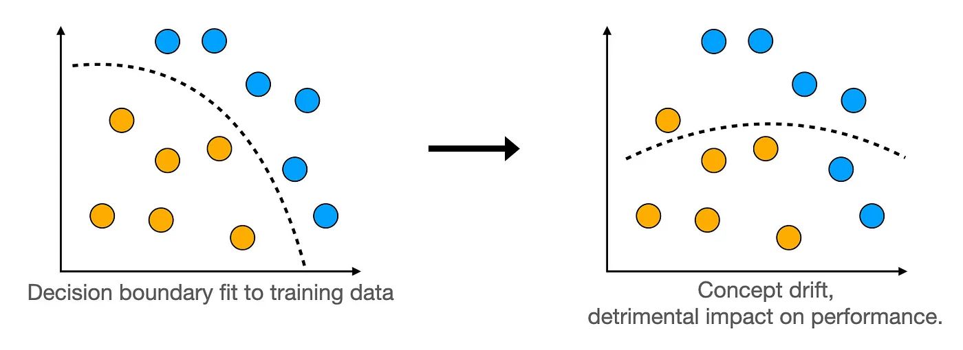
Visualizing concept drift. Image by Michał Oleszak

Consider a default prediction model. During economic hardship, people who previously repaid their loans may start to default on them. In this scenario, the distribution of the input features hasn’t changed, but the conditional distribution of the output given an input has changed. This is a mathematical way of saying that while the borrower’s characteristics haven’t changed, their ability to repay their loan has.

Another potential trigger for concept drift is when a model is used on a different population than the one it was trained on. In the population where the model is used to make inferences, people in similar situations might default for reasons not captured by the model's features.

Covariate shift

Covariate shift refers to the phenomenon where the distribution of your model’s features changes while the relationship between the model’s input and output remains the same.

As mentioned earlier, the data used in loan prediction models primarily consists of data about the terms of the loans and data about the borrower. Let’s explore how the distribution of these features can change.

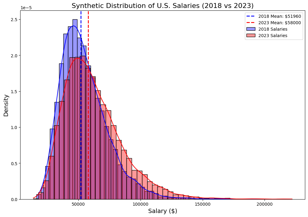
Univariate drift visualised. Plot by author

Changes in loan offerings, such as new installment plans and fluctuating interest rates, can impact the distribution of certain features. Data related to the borrower can also shift. For example, annual income tends to increase yearly due to inflation.

Sometimes, a change in loan offerings can also alter the distribution of some features describing the borrower. For instance, if a bank introduces a new type of low-interest personal loan, it might attract people who previously did not apply for loans, thereby changing the profiles of borrowers.

The above examples relate to shifting trends and changes in the financial and economic landscape; however, covariate shifts can also occur due to changes in data collection. For example, if installments are suddenly reported in the local currency instead of US dollars in the country where the model is used, this would result in a covariate shift. Monitoring for covariate shifts can help explain why your model is failing and allow you to perform the necessary feature engineering to get your model back on track.

Data Quality

Data in default prediction models can come from various sources, including credit bureaus, borrower application forms, and more. This type of data can sometimes be incomplete, which can, in turn, impact the model's performance.

Another challenge related to the data used for default prediction models is that it tends to change. For example, a borrower’s marital status might change, refinancing can alter the loan terms, and job status can shift. These changes are sometimes not communicated to data scientists, possibly leading to degrading models in production.

How to monitor your model

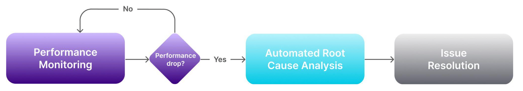
The examples above illustrate just a few of the possible factors that can impact the predictive capability of a default prediction model. NannyML has developed an effective and repeatable workflow that can help you continuously monitor your models in production and prevent these data changes from causing problems for your business.

The method is simple and consists of three steps. The first step involves monitoring the performance of your model. This must be done continuously to ensure that the model is predicting accurately. There is, however, one significant challenge associated with performance monitoring.

NannyML’s performance-centric monitoring workflow

Traditionally, to evaluate a model's performance, you need access to its targets, also known as ground truth, to compare them to the model’s predictions. However, like with many other use cases, for loan default models, we aim to predict whether a borrower will default on their loan ahead of time. If we had access to the actual target, it would defeat the purpose of the model.

For this reason, our team at NannyML has developed performance estimation algorithms that allow you to estimate a model's performance without access to ground truth. For default prediction, which is a classification problem, we can use PAPE, available in NannyML Cloud.

PAPE is an improvement over the CBPE algorithm, which we also developed and made available in our Python open-source library.

Once a performance decrease is detected, the second phase of the model monitoring workflow is put into motion. This phase involves identifying the root cause of the performance drop by detecting concept drift, covariate shift, and data quality issues.

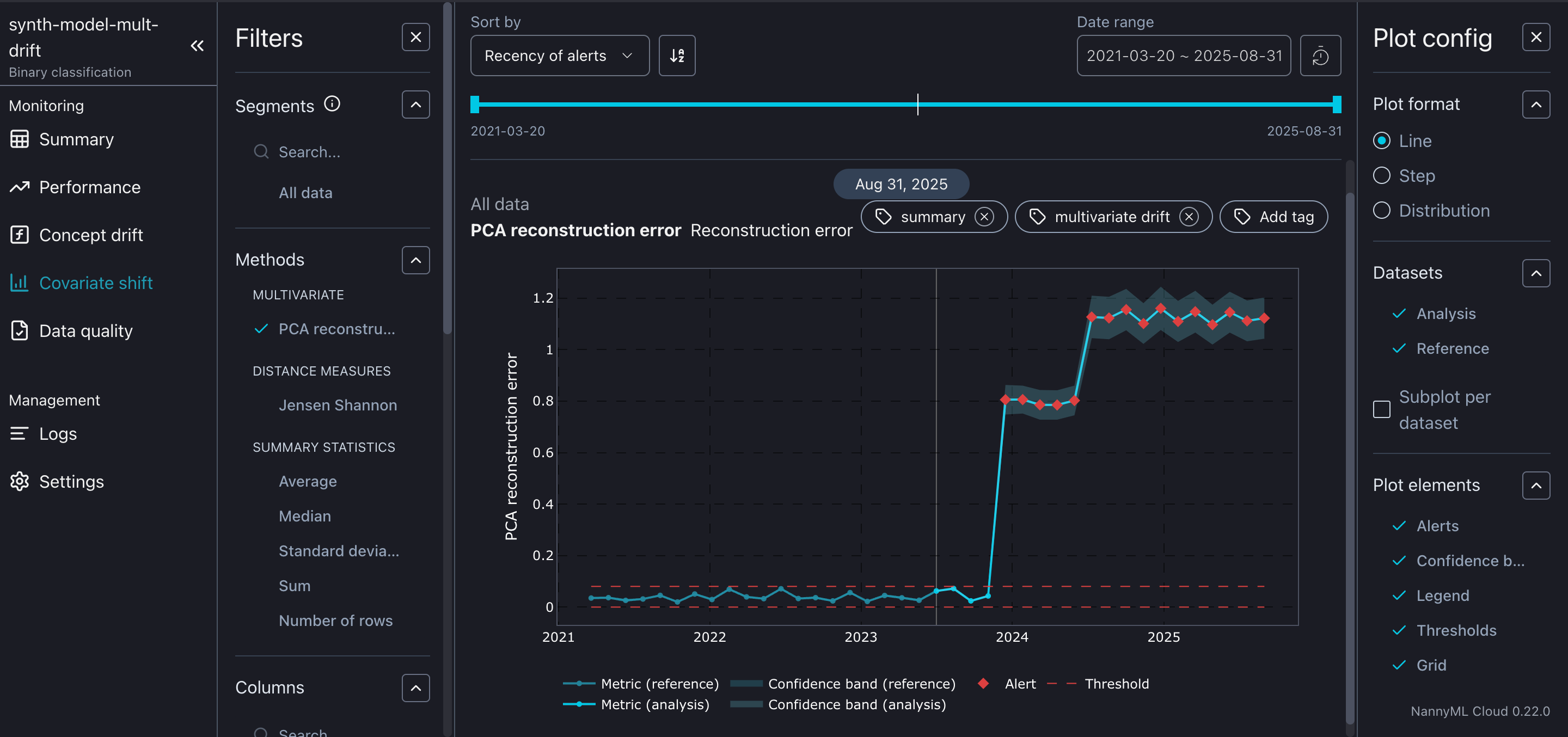
To detect covariate shifts, NannyML has implemented a suite of methods, all of which are described in Kavita's excellent and comprehensive blog. Additionally, NannyML Cloud allows you to monitor statistics such as mean, average, and median to gain a deeper understanding of the changes your data is undergoing.

For data quality issues, we recommend monitoring missing values and unseen values. NannyML defines unseen values for categorical features as those encountered in production that were not present during training.

Finally, concept drift can only be detected when we have access to ground truth. Our team at NannyML developed another method, RCD, for this purpose. It is useful to monitor concept drift once the ground truth becomes available, as it can be a strong indicator that the model needs to be retrained.

Once the root cause of the model failure is detected, it’s time for the final phase of the monitoring workflow: issue resolution. I won’t elaborate on this topic here, as I have written an entire blog on it.

Conclusion

In this blog, we explored the various reasons why default prediction models tend to degrade in production. We then introduced NannyML’s monitoring workflow to demonstrate how to address a failing model. Monitoring an ML model in production is crucial for designing a robust ML system and ensuring that your model delivers optimal value to your organization. This is especially important for a default prediction model, where suboptimal performance can have severe consequences for a financial organization.

NannyML Cloud offers all the necessary tools to effortlessly set up a comprehensive monitoring workflow, ensuring that any declines in your model's performance won't go unnoticed. Sign up for a free trial to discover how NannyML Cloud can benefit your organization.